AC299r: Independent Study
The goal of this independent study is to investigate the lattice Boltzmann method (LBM), a numerical method based on statistical physics and used in computational fluid dynamics, as a preparation to the master’s thesis, “Fluid-Structure Interaction Using the Lattice Boltzmann Method and Reference Map Technique”. The following tasks are completed in this semester:
✅ Built a lattice Boltzmann solver which can handle complex obstacles and simulate turbulent flow.
- Completed a writeup of theory, implementation and validation.
- Simulated two turbulent cases and two obstacle cases. (Jump to see movies!)
✅ Met with Prof. Sauro Succi and discussed preliminary ideas to combine the reference map technique with lattice Boltzmann method.
✅ Studied some introduction to solid mechanics and tensor.
✅ Completed literature review on the lattice Boltzmann method, reference map technique and dissolvable interface between fluid and solid.
|
Reference Map Technique |
|
| 1 |
Rycroft, Chris H., et al. “Reference Map Technique for Incompressible Fluid-Structure Interaction.” ArXiv.org, 6 Oct. 2018, arxiv.org/abs/1810.03015. |
|
Lattice Boltzmann Method and Fluid-Structure Interaction |
|
| 2 |
Succi, Sauro. The Lattice Boltzmann Equation: for Fluid Dynamics and Beyond. Oxford University Press, 2001. |
| 3 | Krüger, Timm & Kusumaatmaja, Halim & Kuzmin, Alexander & Shardt, Orest & Silva, Goncalo & Viggen, Erlend Magnus. (2016). The Lattice Boltzmann Method – Principles and Practice. 10.1007/978-3-319-44649-3. |
| 4 | Rosis, Alessandro De, et al. “Lattice Boltzmann Analysis of Fluid-Structure Interaction with Moving Boundaries.” Communications in Computational Physics, vol. 13, no. 3, 2013, pp. 823–834., doi:10.4208/cicp.141111.201211s. |
| 5 | Benamour, M., et al. “A New Approach Using Lattice Boltzmann Method to Simulate Fluid Structure Interaction.” Energy Procedia, vol. 139, 2017, pp. 481–486., doi:10.1016/j.egypro.2017.11.241. |
| 6 |
Zhang, Raoyang, et al. “Lattice Boltzmann Approach for Local Reference Frames.” Communications in Computational Physics, vol. 9, no. 5, 2011, pp. 1193–1205., doi:10.4208/cicp.021109.111110s. |
| 7 | Tan, Wei, et al. “Fluid-Structure Interaction Using Lattice Boltzmann Method: Moving Boundary Treatment and Discussion of Compressible Effect.” Chemical Engineering Science, vol. 184, 2018, pp. 273–284., doi:10.1016/j.ces.2018.03.042. |
| 8 | Semma, El Alami, et al. “Lattice Boltzmann Method for Melting/Solidification Problems.” Comptes Rendus Mécanique, vol. 335, no. 5-6, 2007, pp. 295–303., doi:10.1016/j.crme.2007.05.015. |
| Dissolving Body in Fluid Flow | |
| 9 | Ristroph, L., et al. “Sculpting of an Erodible Body by Flowing Water.” Proceedings of the National Academy of Sciences, vol. 109, no. 48, 2012, pp. 19606–19609., doi:10.1073/pnas.1212286109. |
| 10 | Moore, Matthew N. J., et al. “Self-Similar Evolution of a Body Eroding in a Fluid Flow.” Physics of Fluids, vol. 25, no. 11, 2013, p. 116602., doi:10.1063/1.4829644. |
| 11 | Huang, Jinzi Mac, et al. “Shape Dynamics and Scaling Laws for a Body Dissolving in Fluid Flow.” Journal of Fluid Mechanics, vol. 765, 2015, doi:10.1017/jfm.2014.718. |
| 12 | Wykes, Megan S. Davies, et al. “Self-Sculpting of a Dissolvable Body Due to Gravitational Convection.” Physical Review Fluids, vol. 3, no. 4, 2018, doi:10.1103/physrevfluids.3.043801. |
| 13 | Rycroft, Chris H., and Martin Z. Bazant. “Asymmetric Collapse by Dissolution or Melting in a Uniform Flow.” Proceedings of the Royal Society A: Mathematical, Physical and Engineering Science, vol. 472, no. 2185, 2016, p. 20150531., doi:10.1098/rspa.2015.0531. |
| Dissolution in Statistical Physics | |
| 14 | Sander, Leonard M. “Diffusion-Limited Aggregation: A Kinetic Critical Phenomenon?” Contemporary Physics, vol. 41, no. 4, 2000, pp. 203–218., doi:10.1080/001075100409698. |
| 15 | Davidovitch, Benny, et al. “Average Shape of Transport-Limited Aggregates.” Physical Review Letters, vol. 95, no. 7, 2005, doi:10.1103/physrevlett.95.075504. |
| CNN and Fluid Simulation | |
| 16 | Jonathan Tompson, Kristofer Schlachter, Pablo Sprechmann, and Ken Perlin. 2017. Accelerating eulerian fluid simulation with convolutional networks. In Proceedings of the 34th International Conference on Machine Learning – Volume 70 (ICML’17), Doina Precup and Yee Whye Teh (Eds.), Vol. 70. JMLR.org 3424-3433. |
| 17 | Yang, Cheng, et al. “Data-Driven Projection Method in Fluid Simulation.” Computer Animation and Virtual Worlds, vol. 27, no. 3-4, 2016, pp. 415–424., doi:10.1002/cav.1695. |
| 18 | Chu, Mengyu, and Nils Thuerey. “Data-Driven Synthesis of Smoke Flows with CNN-Based Feature Descriptors.” ACM Transactions on Graphics, vol. 36, no. 4, 2017, pp. 1–14., doi:10.1145/3072959.3073643. |
| Others | |
| 19 | Saye, R. I., and J. A. Sethian. “The Voronoi Implicit Interface Method for Computing Multiphase Physics.” Proceedings of the National Academy of Sciences, vol. 108, no. 49, 2011, pp. 19498–19503., doi:10.1073/pnas.1111557108. |
This independent study is a direct link to the thesis. With all the theory preparations and a basic lattice Boltzmann fluid solver, the next steps are to adjust the reference map technique in the spirit of lattice Boltzmann, and develop a fluid solver which can handle flexible/dissolvable interface in fluid-structure interaction:
- Create a lattice Boltzmann solver of solid and verify the wave propagation in solid.
- Develop an extension of the lattice Boltzmann method for the reference map technique.
- Formulate a physical model for dissolution of a solid.
- Implement the model in a 2D fluid-structure lattice Boltzmann simulation.
The next section is a writeup of the numerical method and some results (movies included).
I. Theory Formulation
The lattice Boltzmann method (LBM) is based on the Boltzmann equation, which describes the statistical behavior of a thermodynamic system and dates back to 1872. The idea behind the Boltzmann equation is that particles in the system each have 6 degree of freedom, 3 positions and 3 momenta along the 3 coordinate directions  and
and  . Since molecules of a given type are physically indistinguishable from each other, the system can be described completely by the populations of particles as a function of time and these 6 dimensions in the phase space. The Boltzmann Equation describes the evolution of such a system. The populations of particles change due to three terms: diffusion, collisions and external forces.
LBM is a class of computational fluid dynamics methods for fluid simulation that uses the Boltzmann Equation. Instead of solving the macroscopic quantities in the Navier-Stokes equations, the lattice Boltzmann method reconstructs the fluid motion from the microscopic particle models and the mesoscopic kinetic equations, i.e. the probability distribution of the density, momentum and pressure of the fluid particles. The physical system is discretized, typically on a rectilinear grid and most commonly one with square spacing. Particle velocities are also discretized, with particles allowed to jump from one grid point only to nearby grid points over one simulation step. Therefore LBM can also be viewed as a finite difference method solution for the Boltzmann Equation. Due to its simplicity in handling the pressure term in the Navier-Stokes Equation, LBM has emerged as a favorable tool in simulating complex fluid systems.
For a two dimensional model, a particle is restricted to move only in a possible of 9 directions, including the one staying at rest. These velocities are referred to as the microscopic velocities  where
where  . This model is commonly known as the D2Q9 model.
 (Figure 1:Indices and velocity vectors for D2Q9 lattice Boltzmann model.)
D2Q9 can be parsed as referring to 2 dimensions and 9 discrete velocities with attributes below. The 4 first neighbors have displacement  . The 4 second neighbors follow a similar pattern:
  . These displacements give the respective lattice velocity
  . The total weight of the 4 first neighbors is
  . The total weight of the 4 second neighbors is
  . The sum of all weights of the 9 velocity vectors is strictly 1.
| neighbors | # | velocity  |
weight w |
 |
1 |  |
 |
 |
4 |  |
 |
 |
4 |  |
 |
(Table 1: Attributes of displacements and weights to the D2Q9 velocities.)
The macroscopic fluid density is defined as the sum of all neighboring particle distribution functions, i.e. the zero moment of the  at one lattice,
(1) 
Likewise, the first moment refers to the macroscopic fluid momentum, which is equal to the density times the velocity of all neighbors,
(2) 
Retrieving the macroscopic fluid quantities from the microscopic particle distributions is referred as the hydro step in LBM. In addition, three other key steps are involved: equilibrium, collision and streaming. The state of simulation at a timestep is given by the population of particles,  , where the subscript
  refers to the discrete velocities. The movement of population can be described by the Bhatnagar-Gross-Krook (BGK) update rule:
(3) ![\begin{equation*}f_p(\vec{x}+\Detla t \vec{c}_p, t+\Delta t) = f_p(\vec{x},t)+\omega \Detla \bigg[ f_p^{eq}(\rho,\vec{u}-f_p)(\vec{x},t)+\mbox{w}_p\frac{\vec{c}_p \cdot \vec{g}}{c_s^2} \bigg] \end{equation*}](http://sun-yue.com/wp-content/ql-cache/quicklatex.com-4bc0556df0ec857b2a0efcb0f5750c86_l3.png "Rendered by QuickLaTeX.com")
where all terms from left to right are:
♦
 : the population of the particle
♦
 : the timestep, taken to be 1
♦
 : the velocity vector
♦
 : the relaxation time, which is related to the kinematic viscosity
  by
by 
♦
 : macroscopic fluid quantities, calculated via the hydro step
♦
 : the weight of particles with respect to its neighboring hierarchy
♦
 : the acceleration applied to the body by external forces
♦
 : the speed of sound in dimensionless units on the lattices, equal to a constant (
 )
)
The equilibrium populations can be approximated with a Taylor expansion.
(4) ![\begin{equation*}f_p^{eq}(\rho, \vec{u}) = \mbox{w}_p \rho \bigg[ 1+\frac{\vec{u}\cdot \vec{c}_p}{c_s^2} + \frac{(\vec{u}\cdot \vec{c}_p)^2 - c_s^2\vec{u}^2}{2 c_s^4} \bigg]\end{equation*}](http://sun-yue.com/wp-content/ql-cache/quicklatex.com-4aa51a5bb88cc803637895024bc2b021_l3.png "Rendered by QuickLaTeX.com")
This is the equilibrium step. The resulting
 will match the first two moments, i.e. density
  and velocity
  , but will not match the second moment (energy density) unless the system is at equilibrium. This approximation is valid as long as the system is sufficiently close to equilibrium.
The collision step happens after the equilibrium step in the update of a timestep. It describes how neighboring particle populations interact and how their weights move toward their equilibrium values as a result of collisions. When particles hit each other, momentum is conserved, but some kinetic energy is dissipated as heat or in other forms. The equation for the collision step is
(5) 
where
 is the post-collisional populations. In the streaming step, is moved forward to its next timestep,
 (6) 
Eq.(6) is the Navier-Stokes equations in the spirit of the lattice Boltzmann method. The actual implementation requires some subtle constraints, which to be elaborated in the next section. The algorithm of LBM in a capsule is:
II. Numerical Implementation
1. Grid Setup
Set the simulation grid to be of length  and height
  ,
,  grid points along the
  axis and
  grid points along the
  axis. A total of
  fluid lattices, represented in the black dots, form the simulation grid. An extra layer of buffer is padded to each boundary, represented in the blue crosses. With the boundary buffer, no separate functions are needed to handle the boundaries and corners separately in the stream, collide and set boundary condition steps in Algorithm 1. Hence the total number of lattices in the solver is
  .
.
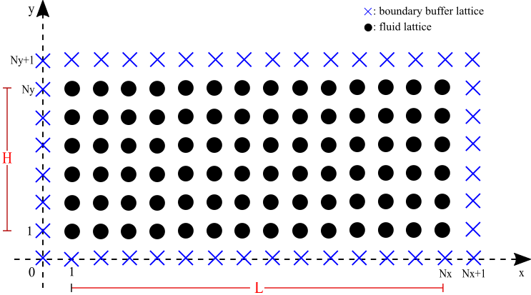
(Figure 2: Two dimensional grid for simulation.)
2. Initial Condition
A common choice is to set the initial density to be uniform and the initial velocity to be zero. Once  and
and  are initialized, a prevalent modeling choice is to initialize the populations to the equilibrium implied by these macroscopic variables, i.e.
(7) 
3. Boundary Condition
Assign each node of the lattices its own specific identity card. Table 2 is an example of a map of a channel flow with  fluid sites, each with its identity card: f: fluid site, w: west boundary buffer, e: east boundary buffer, n: north boundary buffer, s: south boundary buffer, nw: northwest boundary corner, ne: northeast boundary corner, sw: southwest boundary corner, se: southeast boundary corner.
| nw | n | n | n | n | n | n | n | n | n | n | ne |
| w | f | f | f | f | f | f | f | f | f | f | e |
| w | f | f | f | f | f | f | f | f | f | f | e |
| w | f | f | f | f | f | f | f | f | f | f | e |
| w | f | f | f | f | f | f | f | f | f | f | e |
| w | f | f | f | f | f | f | f | f | f | f | e |
| sw | s | s | s | s | s | s | s | s | s | s | se |
(Table 2:Map of a channel flow with identity card.)
- Periodic Boundary Conditions
For simplicity, select periodic conditions at the inlet/outlet and no-slip on the top and bottom rigid walls. Periodicity along is imposed by filling the W buffer with the populations of the rightmost column of the fluid site:(8)

where EF is the eastward fluid row![\mbox{EF} = [i=N; j=1, \cdots, N]](http://sun-yue.com/wp-content/ql-cache/quicklatex.com-890dabba308fe8b9a229d48f6a24324d_l3.png "Rendered by QuickLaTeX.com") and WF is the eastward fluid row
and WF is the eastward fluid row ![\mbox{WF} = [i=N; j=1, \cdots, N]](http://sun-yue.com/wp-content/ql-cache/quicklatex.com-12eb59e7ee40ceaf81dfa9d603880475_l3.png "Rendered by QuickLaTeX.com") . No-slip boundary conditions are implemented by bouncing-back the populations leaving the walls,
. No-slip boundary conditions are implemented by bouncing-back the populations leaving the walls, (9)

where N and S is the top and bottom rows and N-1 and S+1 the immediate lower-lying and upper-lying fluid rows, respectively. The four corners need special handling of the bounceback constraint:(10)

where NW, SW, NE, SE are the northwest, southwest, northeast and southeast boundary corners, and NWF, SWF, NEF, SEF are the corner fluid lattices. Note that this no-slip condition is on-grid, and is only first-order accurate because of the one-sided character of the streaming operator at the boundary. The map that transfers the inward and outward populations, subscripted in “in” and “out”, is:(11)

With the boundary buffer, walls and corners do not need to be handled separately using Zou-He boundary condition. But it is still one out of several possible strategies. - Open Boundary Conditions
Here the open boundary is limited to inlet and outlet situation. For these open flows, it is common to assign a given velocity profile at the inlet while at the outlet either a given pressure
  or a no-flux condition normal to the wall,
  , is imposed. The inlet is implemented by refilling the west boundary buffer with the equilibrium population corresponding to the desired values of density and flow speed at each timestep:
(12)
![\begin{equation*}f_{\mbox{in}}(y) = f^{eq}[\rho_{\mbox{in}}, u_{\mbox{in}}(y)]\end{equation*}](http://sun-yue.com/wp-content/ql-cache/quicklatex.com-7f1fcc4a14403ee3ea5de01a4153f6bc_l3.png "Rendered by QuickLaTeX.com")
For the outlet, there are two possible schemes. First, if the outlet is placed for enough downstream so as to allow the flow settle down to a one-dimensional zero-gradient profile, the outlet can simply be copied from the eastward fluid column. If this condition is not met, then backward propagating disturbances would occur and destroy the simulation. The second approach is to apply a “porous plug” boundary condition at the outlet buffer, that the particles reading the outlet are reflected back with a probability , which ensures mass conservation:
(13)

4. Stream
This step pulls the contribution from neighboring lattices and update the lattice of interest, therefore it is not a local operation. In lbm.cc, for each fluid lattice on the simulation grid,
(14) 
where left, down, right, up, bottom left, bottom right, top right and top left represent the direction of the neighboring lattices to the lattice of interest. This operation is valid even for fluid lattices near the boundary because of the boundary buffer.
[Add image]
5. Hydro
This operation of retrieving macroscopic hydrodynamic quantities is local to each fluid lattice . In lattice.hh, calculate the zero and first moments of the 9 populations  :
:
(15) 
6. Equilibrium
The equilibrium step is also local to each fluid lattice. Eq.(5) has an alternative form,
(16) ![\begin{equation*}f_i^{eq} = \rho \mbox{w}_i [1 + \frac{c_{ia}\vec{u}_a}{c_s^2} + \frac{Q_{iab}\vec{u}_a\vec{u}_b}{2c_s^4}]\end{equation*}](http://sun-yue.com/wp-content/ql-cache/quicklatex.com-c10d0a5bca31c3412a9d2eec76cfbdfe_l3.png "Rendered by QuickLaTeX.com")
Explicitly,
(17) 
7. Collide
This step of updating the fluid lattice populations is also local to each fluid lattice:
(18) 
III. Results
The lattice Boltzmann fluid solver is supposed to be robust and efficient since it does not require the projection step in traditional computational fluid dynamics, i.e. solving a Laplacian equation for the pressure. Two test cases are presented to show how this solver can be used to simulate complex geometry and turbulence.
Two variables control the simulation, the Reynolds number  and the relaxation time
  . A larger Reynolds number or a relaxation number closer to 0.5 correspond to turbulent flow.
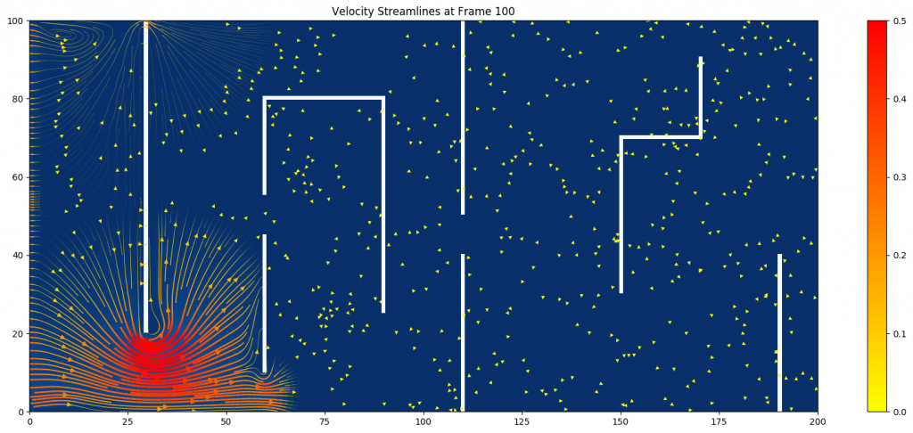
Case 1: Simulate a flow through a maze
1.1 Simulation parameters: 
The movie shows a quiescent flow development through a maze-like channel. The channel has no-slip top and bottom, with an inlet plug flow with  and an outlet. The brighter color represents higher velocity, and the flow finds its optimal path through the channel. It shows the potential of a fluid solver in visualizing the optimal maze path.
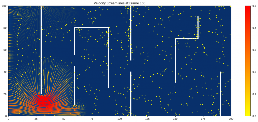
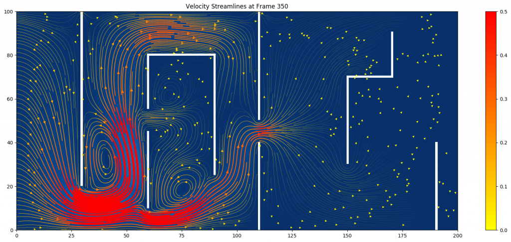
(Figure 3: Velocity streamlines at  )
)
The velocity streamlines offer a better visualization of the subtle motion of the flow. The denser and more red streamlines represent higher velocity magnitude, which cluster around the narrowings. In addition, many circulations and swirlings happen between obstacle plates.
1.2 Simulation parameters: 
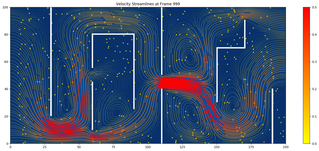
The movie shows the same simulation setting only with a smaller relaxation time. In this case the fluid moves faster, and more turbulence and circulations occur in the system.
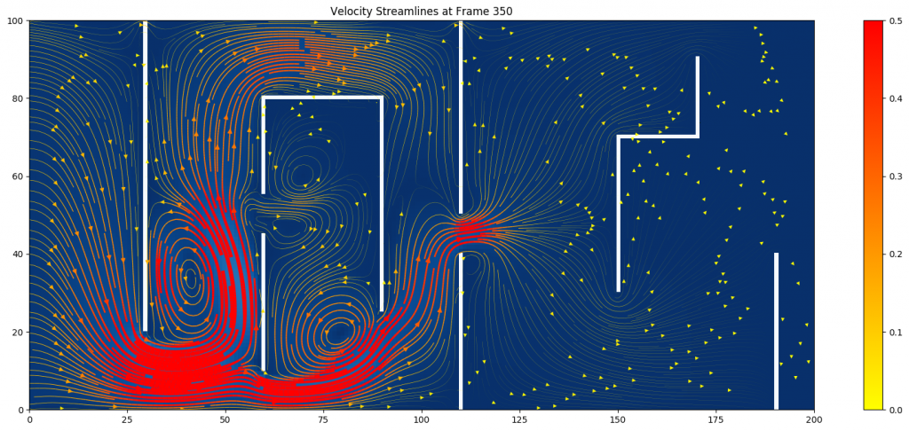
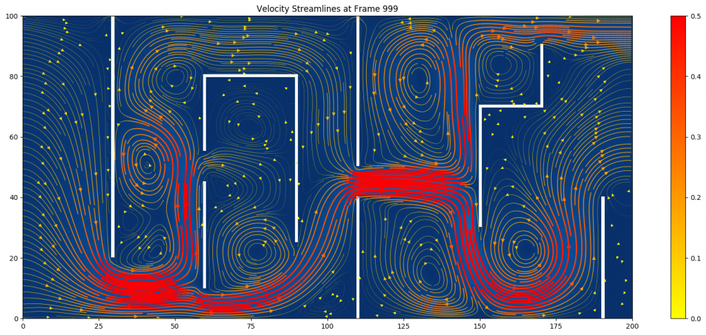 (Figure 3: Velocity streamlines at )
At the same simulation time, the flow moves faster and has more circulations in the system with a smaller relaxation time. This corresponds to the fact that the relaxation time controls how turbulent the system is.
Case 2: Simulate a simple von Karmen vortex
Simulation parameters: 
This movie is a vorticity evolution with respect to time of a von Karmen vortex simulation. The channel has no-slip top and bottom, with an inlet plug flow with and an outlet.